Filter operations are very common in computer vision applications and are often the first operations applied to an image. Blur, sharpen or gradient filters are common examples. Mathematically, the underlying operation is called convolution and already covered in a separate article. The good thing is that filter operations are very well suited for parallel computing and hence can be executed very fast on the GPU. I worked recently on a GPU-project were the filter operations made up the dominant part of the complete application and hence got first priority in the optimization phase of the project. In this article, I want to share some of the results.
First, a few words about GPU programming1. The GPU is very different from the CPU since it serves a completely different purpose (mainly gaming). This results in a completely different architecture and design principles. A GPU is a so-called throughput-oriented device where the goal is to execute many, many tasks concurrently on the processing units. Not only that a GPU has much more processing units than a CPU, it is also designed to leverage massive parallelism, e.g. by the concept of additional hardware threads per core. Just as a comparison: the CPU is a latency-oriented device. Its main goal is to execute a single task very fast, e.g. by introducing fast memory caching mechanism.
The demanding task for the developer is to keep the GPU busy. This is only possible by exploiting the parallelism of the application and optimize the code regarding this subject. One important factor, and as I now learned the important factor, which stalls the GPU is memory access. Since the GPU has a lot of processing units it needs also more memory to serve the units with data. Unlike to the CPU, it is under control of the developer where to store the memory which offers great flexibility and an additional degree of freedom in the optimization process. Badly designed memory transfers, e.g. by repeatedly copying data from the global to the private memory of the work-items, can take up most of the execution time.
As you may already have guessed from the title, I use OpenCL as a framework in version 2.0 and all the tests are run on an AMD R9 2902 @ 1.1 GHz GPU. Scharr filter (gradient filter) in the horizontal and vertical direction
\begin{equation} \label{eq:FilterOptimization_ScharrFilter} \partial_x = \begin{pmatrix} -3 & 0 & 3 \\ -10 & {\color{Aquamarine}0} & 10 \\ -3 & 0 & 3 \\ \end{pmatrix} \quad \text{and} \quad \partial_y = \begin{pmatrix} -3 & -10 & -3 \\ 0 & {\color{Aquamarine}0} & 0 \\ 3 & 10 & 3 \\ \end{pmatrix} \end{equation}are used as filter kernel (centre position highlighted) and applied to an image pyramid consisting of four octaves with four images each3. Every benchmark measures how fast the two filters can be applied to the complete pyramid averaged over 20 runs. Note, that the creation of the pyramid (including the initial image transfer to the GPU) or the compilation time of the kernels is not included. I only want to measure the impact of the filter operation. Since the size of the filter is also very important, four different dimensions are used: \(3 \times 3\), \(5 \times 5\), \(7 \times 7\) and \(9 \times 9\). Filters larger than \(3 \times 3\) are basically \eqref{eq:FilterOptimization_ScharrFilter} scaled up but with slightly different numbers. In any case, there are only six non-zero entries. Filters are stored in float* arrays and the image itself is a grey-scale image converted to floating data type, i.e. the OpenCL data type image2d_t is used.
I want to assess the performance of filter operations in five test cases:
- Single: filter operation without further optimizations.
- Local: the image data is cached in local memory to exploit the fact that each pixel is needed multiple times.
- Separation: both filters in \eqref{eq:FilterOptimization_ScharrFilter} are linearly separable. In this case, it is possible to split up each filter in a horizontal and vertical vector and apply them to the image in two passes.
- Double: \(\partial_x\) and \(\partial_y\) are independent of each other. Since usually the response from both filters is needed and both are applied to the same image, it is possible to write an optimized kernel for that case.
- Predefined: Scharr filters are very common and it is likely that we need them multiple times. We could write a specialized kernel just for Scharr filters without the need to pass the filter as a parameter to the kernel. We can even go one step further and take the values of the filter into account, e.g. by omitting zero entries.
I don't have an extra case where I put the filter in constant memory since this is an optimization which I already implemented in the beginning (it is not very hard since the only thing to do is to declare the parameter pointing to the filer as constant float* filter), so the usage of constant memory is always included. Another common optimization is filter unrolling where the filter size must be known at compile time. The compiler can then produce code containing the complete filter loop as explicit steps without introducing the loop overhead (e.g. conditional checks if the loop has ended). Since this is also something where every test case benefits from, it is included, too.
Note also that these cases are not independent of each other. It is e.g. possible to use local memory and separate the filter. This makes testing a bit complicated since there are a lot of combinations possible. I start by considering each case separately and look at selected combinations at the end. All code which I used here for testing is also available on GitHub.
The next sections will cover each of the test cases in more detail, but the results are already shown in the next figure so that you can always come back here to compare the numbers.
Single
The basic filter operation without any optimizations is implemented straightforwardly in OpenCL. We centre our Scharr filter at the current pixel location and then perform the convolution. The full code is shown as it serves as the basis for the other test cases.
/**
 * Calculates the filter sum at a specified pixel position. Supposed to be called from other kernels.
 *
 * Additional parameters compared to the base function (filter_single_3x3):
 * @param coordBase pixel position to calculate the filter sum from
 * @return calculated filter sum
 */
float filter_sum_single_3x3(read_only image2d_t imgIn,
                            constant float* filterKernel,
                            const int2 coordBase,
                            const int border)
{
    float sum = 0.0);
    const int rows = get_image_height(imgIn);
    const int cols = get_image_width(imgIn);
    int2 coordCurrent;
    int2 coordBorder;
    float color;

    // Image patch is row-wise accessed
    // Filter kernel is centred in the middle
    #pragma unroll
    for (int y = -ROWS_HALF_3x3; y <= ROWS_HALF_3x3; ++y)       // Start at the top left corner of the filter
    {
        coordCurrent.y = coordBase.y + y;
        #pragma unroll
        for (int x = -COLS_HALF_3x3; x <= COLS_HALF_3x3; ++x)   // And end at the bottom right corner
        {
            coordCurrent.x = coordBase.x + x;
            coordBorder = borderCoordinate(coordCurrent, rows, cols, border);
            color = read_imagef(imgIn, sampler, coordBorder).x;

            const int idx = (y + ROWS_HALF_3x3) * COLS_3x3 + x + COLS_HALF_3x3;
            sum += color * filterKernel[idx];
        }
    }

    return sum;
}

/**
 * Filter kernel for a single filter supposed to be called from the host.
 *
 * @param imgIn input image
 * @param imgOut image containing the filter response
 * @param filterKernel 1D array with the filter values. The filter is centred on the current pixel and the size of the filter must be odd
 * @param border int value which specifies how out-of-border accesses should be handled. The values correspond to the OpenCV border types
 */
kernel void filter_single_3x3(read_only image2d_t imgIn,
                              write_only image2d_t imgOut,
                              constant float* filterKernel,
                              const int border)
{
    int2 coordBase = (int2)(get_global_id(0), get_global_id(1));

    float sum = filter_sum_single_3x3(imgIn, filterKernel, coordBase, border);

    write_imagef(imgOut, coordBase, sum);
}
The sampler is a global object. Also, borderCoordinate() is a helper function to handle accesses outside the image border. Both definitions are not shown here and I refer to the full implementation (both are defined in filter.images.cl) for further interest, but it is not important here for the tests. We can call the filter_single_3x3() kernel from the host with the cl::NDRange set to the image size of the current level in the pyramid, e.g. something like
//...
const size_t rows = imgSrc.getImageInfo<CL_IMAGE_HEIGHT>();
const size_t cols = imgSrc.getImageInfo<CL_IMAGE_WIDTH>();

imgDst = std::make_shared<cl::Image2D>(*context, CL_MEM_READ_WRITE, cl::ImageFormat(CL_R, CL_FLOAT), cols, rows);

cl::Kernel kernel(*program, "filter_single_3x3");
kernel.setArg(0, imgSrc);
kernel.setArg(1, *imgDst);
kernel.setArg(2, bufferKernel1);    // {-3, 0, 3, -10, 0, 10, -3, 0, 3}
kernel.setArg(3, border);           // BORDER_REPLICATE (aaa|abcd|ddd)

const cl::NDRange global(cols, rows);
queue->enqueueNDRangeKernel(kernel, cl::NullRange, global, cl::NullRange);
The needed filter sizes need to be defined correctly, e.g.
#define COLS_3x3 3
#define COLS_HALF_3x3 1
#define ROWS_HALF_3x3 1
with the half versions calculated with int cast, i.e. \(rowsHalf = \left\lfloor \frac{rows}{2} \right\rfloor\). They need to be set as defines so that #pragma unroll can do its job. As you can see from the test results, this solution is not very fast compared to the others. This is good news since there is still room for optimizations.
Local
In the filter operation, each pixel is accessed multiple times by different work-items due to the incorporation of the neighbourhood in the convolution operation. It is not very efficient to transfer the data again and again from global to private memory since access to global memory is very slow. The idea is to cache the image's pixel values in local memory and access it from here. This reduces the need for global memory transfers significantly.
Local memory is attached to each compute unit on the GPU and is shared between work-groups. Work-groups on different compute units can't share the same data, so the caching is restricted to the current work-group. Since the work-group size is limited, e.g. to \(16 \times 16\) on the AMD R9 290 GPU, we need to split up the image into \(16 \times 16\) blocks. Each work-group must copy the parts of the image it needs into its own local memory. This would be easy if a work-group would only need to access data from its own \(16 \times 16\) image block. But the incorporation of the neighbourhood also holds for the border pixels, so we need to copy a bit more than \(16 \times 16\) pixels from the image depending on the filter size. E.g. for a \(3 \times 3\) filter a 1 px wide padding is needed.
Ok, we just need to copy a few more pixels, shouldn't be a problem, should it? It turns out that this is indeed a bit tricky. The problem is: which work-items in the work-group copy which pixels? We need to define a pattern and write it down as (messy) index calculation in code. To make things a bit simpler, consider the following example of a \(16 \times 16\) block which is located somewhere around the top left corner.
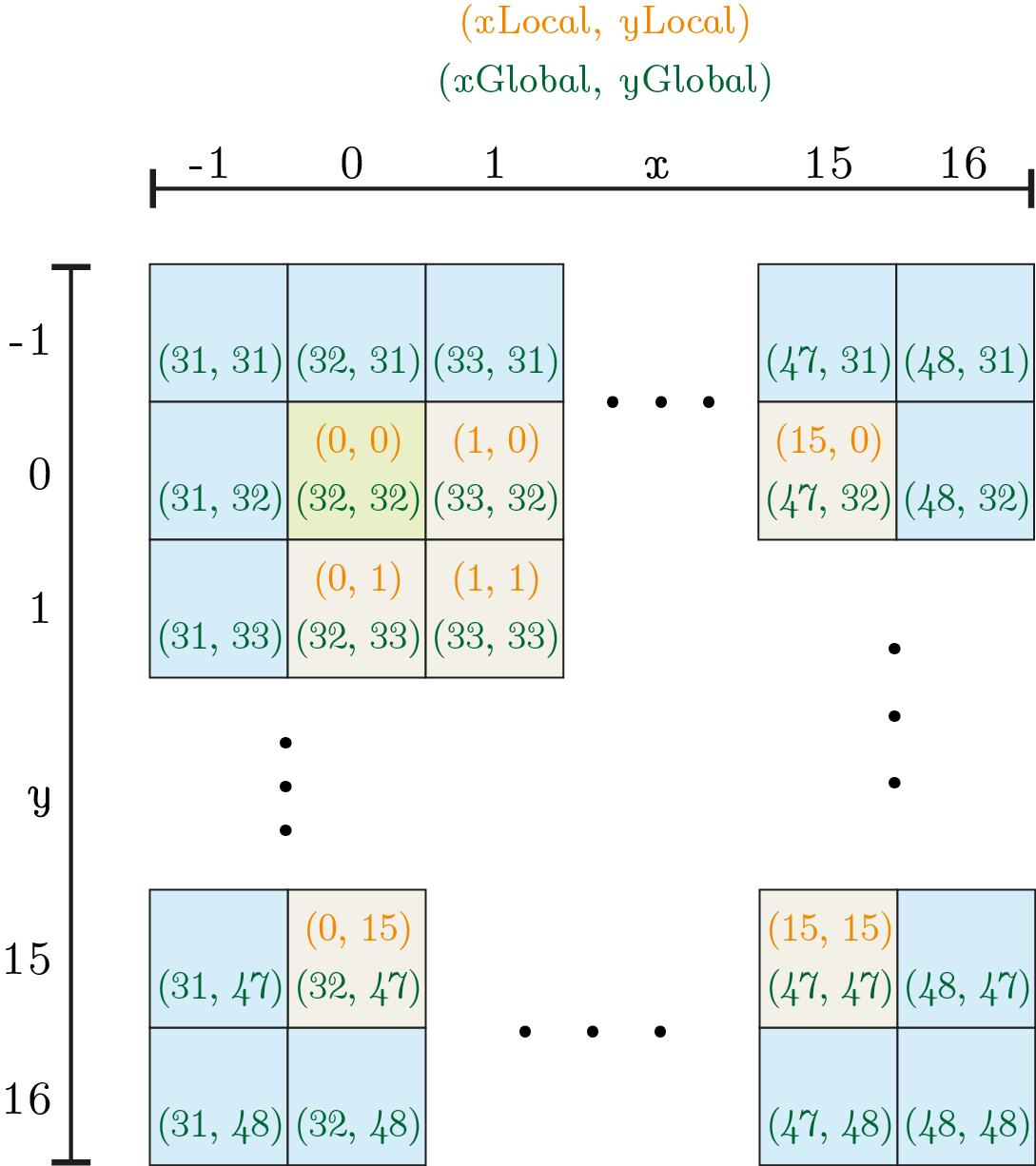
for loop of the next listing. Inside the pixels, the top index \({\color{Orange}(x_{local},y_{local})}\) shows the local id and the bottom index pair \({\color{Green}(x_{global},y_{global})}\) the global id used in this example. Blue pixels are needed for padding to allow correct filter calculations of the border pixels. The green pixel in the top left corner of the patch marks the base pixel.First, note that the size of the local buffer must be large enough to cover all pixels shown. The idea is then to iterate over the local buffer (outer index), map the calculation relative to the base pixel and then copy the data according to the current outer pixel. Usually, this involves 4 iterations where we start with a \(16 \times 16\) block in the top left corner and move on in a zigzag fashion to gather the remaining pixels as shown in the following figure.
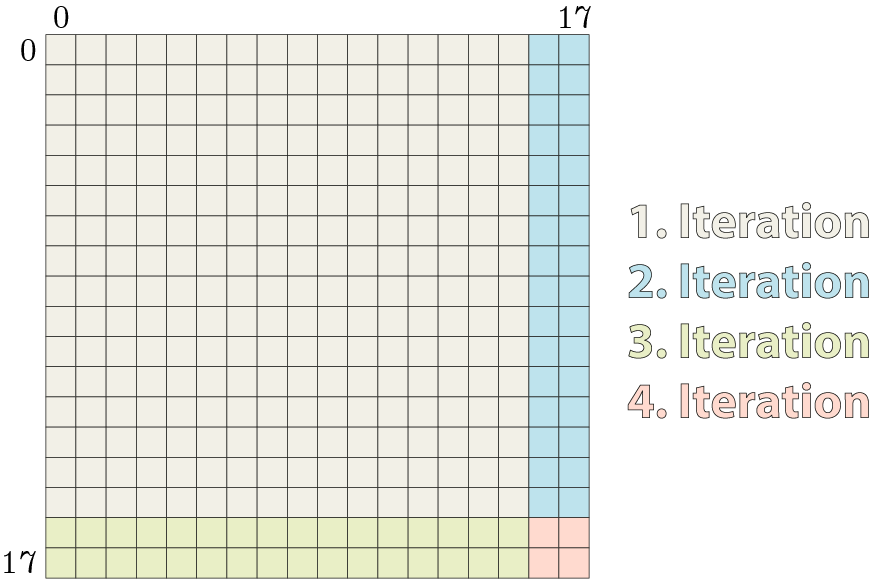
Except for the first iteration and not too large filter sizes, not all of the 256 work-items are busy during this calculation. Especially the fourth iteration where only 4 of the 256 work-items do something useful is not beautiful to look at4. But since the local buffer size does not map perfectly with the size of the work-group, this is unavoidable with this pattern. Implementing it results in:
/**
 * Calculates the filter sum using local memory at a specified pixel position. Supposed to be called from other kernels.
 *
 * Additional parameters compared to the base function (filter_single_local_3x3):
 * @param coordBase pixel position to calculate the filter sum from
 * @return calculated filter sum
 */
float filter_sum_single_local_3x3(read_only image2d_t imgIn,
                                  constant float* filterKernel,
                                  int2 coordBase,
                                  const int border)
{
    const int rows = get_image_height(imgIn);
    const int cols = get_image_width(imgIn);

    // The exact size must be known at compile time (no dynamic memory allocation possible)
    // Adjust according to the highest needed filter size or set via compile parameter
    local float localBuffer[LOCAL_SIZE_COLS_3x3 * LOCAL_SIZE_ROWS_3x3];   // Allocate local buffer

    int xLocalId = get_local_id(0);
    int yLocalId = get_local_id(1);

    int xLocalSize = get_local_size(0);
    int yLocalSize = get_local_size(1);

    // The top left pixel in the current patch is the base for every work-item in the work-group
    int xBase = coordBase.x - xLocalId;
    int yBase = coordBase.y - yLocalId;

#if COLS_3x3 >= 9 || ROWS_3x3 >= 9
    /*
     * Copy the image patch including the padding from global to local memory. Consider for example a 2x2 patch with a padding of 1 px:
     * bbbb
     * bxxb
     * bxxb
     * bbbb
     * The following pattern fills the local buffer in 4 iterations with a local work-group size of 2x2
     * 1122
     * 1122
     * 3344
     * 3344
     * The number denotes the iteration when the corresponding buffer element is filled. Note that the local buffer is filled beginning in the top left corner (of the buffer)
     *
     * Less index calculation but more memory accesses, better for larger filter sizes
     */
    for (int y = yLocalId; y < yLocalSize + 2 * ROWS_HALF_3x3; y += yLocalSize)
    {
        for (int x = xLocalId; x < xLocalSize + 2 * COLS_HALF_3x3; x += xLocalSize)
        {
            // Coordinate from the image patch which must be stored in the current local buffer position
            int2 coordBorder = borderCoordinate((int2)(x - COLS_HALF_3x3 + xBase, y - ROWS_HALF_3x3 + yBase), rows, cols, border);
            localBuffer[y * LOCAL_SIZE_COLS_3x3 + x] = read_imagef(imgIn, sampler, coordBorder).x;   // Fill local buffer
        }
    }
#else
    /*
     * Copy the image patch including the padding from global to local memory. The local ID is mapped to the 1D index and this index is remapped to the size of the local buffer. It only needs 2 iterations
     *
     * More index calculations but less memory accesses, better for smaller filter sizes (a 9x9 filter is the first which needs 3 iterations)
     */
    for (int idx1D = yLocalId * xLocalSize + xLocalId; idx1D < (LOCAL_SIZE_COLS_3x3 * LOCAL_SIZE_ROWS_3x3); idx1D += xLocalSize * yLocalSize) {
        int x = idx1D % LOCAL_SIZE_COLS_3x3;
        int y = idx1D / LOCAL_SIZE_COLS_3x3;

        // Coordinate from the image patch which must be stored in the current local buffer position
        int2 coordBorder = borderCoordinate((int2)(x - COLS_HALF_3x3 + xBase, y - ROWS_HALF_3x3 + yBase), rows, cols, border);
        localBuffer[y * LOCAL_SIZE_COLS_3x3 + x] = read_imagef(imgIn, sampler, coordBorder).x;   // Fill local buffer
    }
#endif

    // Wait until the image patch is loaded in local memory
    work_group_barrier(CLK_LOCAL_MEM_FENCE);

    // The local buffer includes the padding but the relevant area is only the inner part
    // Note that the local buffer contains all pixels which are read but only the inner part contains pixels where an output value is written
    coordBase = (int2)(xLocalId + COLS_HALF_3x3, yLocalId + ROWS_HALF_3x3);
    int2 coordCurrent;
    float color;
    float sum = 0.0f;

    // Image patch is row-wise accessed
    #pragma unroll
    for (int y = -ROWS_HALF_3x3; y <= ROWS_HALF_3x3; ++y)
    {
        coordCurrent.y = coordBase.y + y;
        #pragma unroll
        for (int x = -COLS_HALF_3x3; x <= COLS_HALF_3x3; ++x)
        {
            coordCurrent.x = coordBase.x + x;
            color = localBuffer[coordCurrent.y * LOCAL_SIZE_COLS_3x3 + coordCurrent.x];    // Read from local buffer

            const int idx = (y + ROWS_HALF_3x3) * COLS_3x3 + x + COLS_HALF_3x3;
            sum += color * filterKernel[idx];
        }
    }

    return sum;
}
The relevant part is located at the lines 46–54. Notice how x - COLS_HALF_3x3 maps to the outer index shown in the example and when this is added to the base pixel we cover the complete local buffer. For example, the work-item \(w_1 = {\color{Orange}(0, 0)}\) executes the lines in its first iteration as
int2 coordBorder = borderCoordinate((int2)(0 - 1 + 32, 0 - 1 + 32) /* = (31, 31) */, rows, cols, border);
localBuffer[0 * 18 + 0] = read_imagef(imgIn, sampler, coordBorder).x;
which copies the top left pixel to the first element in the local buffer. Can you guess which second pixel the same work-item copies in its second iteration?5
When working with local buffers there is one caveat: the size of the buffer must be known at compile time and it is not possible to allocate it dynamically. This means that the defines
#define LOCAL_SIZE_COLS_3x3 18 // 16 + 2 * 1
#define LOCAL_SIZE_ROWS_3x3 18 // 16 + 2 * 1
must be set properly before using this function. This becomes less of a problem when loop unrolling is used (like here) since then the filter size must be known anyway.
Skip the second #else pragma for now and consider line 76ff where the base index is calculated. This adds the padding to the local id since we need only calculate the filter responses of the inner block (the padding pixels are only read, not written). For example, the work-item \(w_1\) sets this to
int2 coordBaseLocal = (int2)(0 + 1, 0 + 1) /* = (1, 1) */;
and accesses later the top left pixel in its first iteration (since the filter is centred at \({\color{Orange}(0, 0)}\))
// Image patch is row-wise accessed
#pragma unroll
for (int y = -1; y <= 1; ++y)
{
    coordCurrent.y = 1 + -1;
    #pragma unroll
    for (int x = -1; x <= 1; ++x)
    {
        coordCurrent.x = 1 + -1;
        float color = localBuffer[0 * 18 + 0];    // Read from local buffer

        const int idx = (-1 + 1) * 3 + -1 + 1;
        sum += color * filterKernel[0];
    }
}
The access pattern shown in the lines 46–54 has the disadvantage that it needs at least 4 iterations even though a \(3 \times 3\) filter can theoretically fetch all data in two iterations (256 inner pixels and \(16*1*4 + 1*1*4 = 68\) padding pixels). Therefore, I also implemented a different approach (lines 61–68). The idea here is to map the index range of the local ids of the \(16 \times 16\) block to a 1D index and then remap them back to the local buffer size. This is also visualized in the following figure.
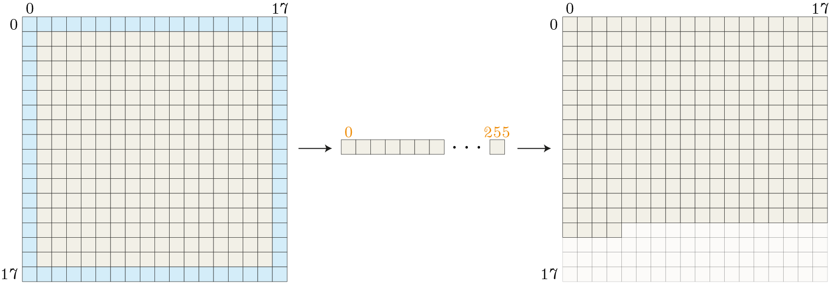
For the work-item \(w_{18} = {\color{Orange}(1, 1)}\) lines 61–68 expand to
for (int idx1D = 1 * 16 + 1 /* = 17 */; idx1D < (18 * 18 /* = 324 */); idx1D += 16 * 16 /* = 256 */) {
    int x = 17 % 18 /* = 17 */;
    int y = 17 / 18 /* = 0 */;

    // Coordinate from the image patch which must be stored in the current local buffer position
    int2 coordBorder = borderCoordinate((int2)(17 - 1 + 32, 0 - 1 + 32) /* = (48, 31) */, rows, cols, border);
    localBuffer[0 * 18 + 17] = read_imagef(imgIn, sampler, coordBorder).x;   // Fill local buffer
}
and issues a copy operation for the top right pixel from global memory into the local buffer. Even though this approach results in fewer iterations it comes at the cost of higher index calculations. Comparing the two approaches shows only a little difference in the beginning.
for loops (lines 46–54) and the orange line denotes the results when using just 1 for loop but more index calculations (lines 61–68).Only for a \(7 \times 7\) filter there is a small advantage of \(\approx 1.5\,\text{ms}\) for the index remapping approach. It is very noticeable though that a \(9 \times 9\) filter is much faster in the 2-loops approach. This is the first filter which needs 3 iterations in the remapping approach (256 inner pixels and \(16*4*4+4*4*4=320>256\)) and the critical point where the overhead of the index calculations gets higher than the cost of the additional iteration in the 2-loop approach.
Even though the difference is not huge, I decided to use the remapping approach for filter sizes up to \(7 \times 7\) and the 2-loop approach otherwise (hence the #if pragma).
Comparing the use of local memory with the other test cases shows that local memory gets more efficient with larger filter sizes. In the case of a \(3 \times 3\) filter the results are even a little bit worse due to the overhead of copying the data from global to local memory. But for the other filter sizes, this is definitively an optimization we should activate.
Separation
Separation is an optimization which does not work with every filter. To apply this technique, it must be possible to split up the filter in one column and one row vector so that their outer product results in the filter again, e.g. for a \(3 \times 3\) filter the equation
\begin{align*} H &= \fvec{a} \cdot \fvec{b} \\ \begin{pmatrix} h_{11} & h_{12} & h_{13} \\ h_{21} & h_{22} & h_{23} \\ h_{31} & h_{32} & h_{33} \\ \end{pmatrix} &= \begin{pmatrix} a_1 \\ a_2 \\ a_3 \\ \end{pmatrix} \cdot \begin{pmatrix} b_1 & b_2 & b_3 \\ \end{pmatrix} \end{align*}must hold. Luckily, this is true for our Scharr filter
\begin{align*} \partial_x &= \fvec{\partial}_{x_1} \cdot \fvec{\partial}_{x_1} \\ \begin{pmatrix} -3 & 0 & 3 \\ -10 & 0 & 10 \\ -3 & 0 & 3 \\ \end{pmatrix} &= \begin{pmatrix} -3 \\ -10 \\ -3 \\ \end{pmatrix} \cdot \begin{pmatrix} 1 & 0 & -1 \\ \end{pmatrix}. \end{align*}How does this help us? Well, we can use this when performing the convolution operation with the image \(I\)
\begin{equation*} I * \partial_x = I * \fvec{\partial}_{x_1} * \fvec{\partial}_{x_2} = I * \fvec{\partial}_{x_2} * \fvec{\partial}_{x_1}. \end{equation*}So, we can perform two convolutions instead of one and the order doesn't matter. This is interesting because we now perform two convolutions with a \(3 \times 1\) respectively a \(1 \times 3\) filter instead of one convolution with a \(3 \times 3\) filter. The benefit may be not so apparent for such a small filter but for larger filters, this gives us the opportunity to save a lot of computations. However, we also increase the memory consumption due to the need for a temporary image which is especially crucial on GPUs, as we will see.
But first, let's look at a small example. For this, consider the following definition of \(I\)
\begin{equation*} I = \begin{pmatrix} 0 & 1 & 0 & 1 \\ 2 & 2 & 0 & 0 \\ 0 & {\color{Aquamarine}3} & 1 & 0 \\ 0 & 1 & 0 & 0 \\ \end{pmatrix} \end{equation*}where the convolution at the highlighted position is calculated as (note that the filter is swapped in the convolution operation)
\begin{equation*} (I * \partial_x)(2, 3) = 2 \cdot 3 + (-10) \cdot 1 = -4. \end{equation*}To achieve the same result with separation we also need the horizontal neighbours of our element and apply the column-vector
\begin{align*} (I * \fvec{\partial}_{x_1})(1, 3) &= 2 \cdot (-3) + 0 \cdot (-10) + 0 \cdot (-3) = -6 \\ (I * \fvec{\partial}_{x_1})(2, 3) &= 2 \cdot (-3) + 3 \cdot (-10) + 1 \cdot (-3) = -39 \\ (I * \fvec{\partial}_{x_1})(3, 3) &= 0 \cdot (-3) + 1 \cdot (-10) + 0 \cdot (-3) = -10. \end{align*}These are our temporary values where we would need a temporary image with the same size as the original image during the filter process. Next, apply the column vector on the previous results
\begin{equation*} \left( (I * \fvec{\partial}_{x_1}) * \fvec{\partial}_{x_2} \right)(2, 3) = (-6) \cdot (-1) + (-39) \cdot 0 + (-10) \cdot 1 = -4 \end{equation*}and we get indeed the same result. If you want to see the full example, check out the attached Mathematica notebook.
The kernel code which implements separate filter convolution is not too different from the single approach. It is basically the same function, just using different defines
#define COLS_1x3 3
#define COLS_HALF_1x3 1
#define ROWS_1x3 1
#define ROWS_HALF_1x3 0
and adjust the names in the kernel definition accordingly
float filter_sum_single_1x3(read_only image2d_t imgIn,
                            constant float* filterKernel,
                            const int2 coordBase,
                            const int border)
{
    //...
    #pragma unroll
    for (int y = -ROWS_HALF_1x3; y <= ROWS_HALF_1x3; ++y)       // Start at the top left corner of the filter
    {
        coordCurrent.y = coordBase.y + y;
        #pragma unroll
        for (int x = -COLS_HALF_1x3; x <= COLS_HALF_1x3; ++x)   // And end at the bottom right corner
        {
            //...
            const int idx = (y + ROWS_HALF_1x3) * COLS_1x3 + x + COLS_HALF_1x3;
            sum += color * filterKernel[idx];
        }
    }

    return sum;
}
But from the host side, we need to call two kernels, e.g. something like
//...
cl::Image2D imgTmp(*context, CL_MEM_READ_WRITE, cl::ImageFormat(CL_R, CL_FLOAT), cols, rows);
imgDst = std::make_shared<cl::Image2D>(*context, CL_MEM_READ_WRITE, cl::ImageFormat(CL_R, CL_FLOAT), cols, rows);

cl::Kernel kernelX(*program, "filter_single_1x3");
kernelX.setArg(0, imgSrc);
kernelX.setArg(1, imgTmp);
kernelX.setArg(2, bufferKernelSeparation1A);    // (-3, -10, -3)^T
kernelX.setArg(3, border);

cl::Kernel kernelY(*program, "filter_single_3x1");
kernelY.setArg(0, imgTmp);
kernelY.setArg(1, *imgDst);
kernelY.setArg(2, bufferKernelSeparation1B);    // (1, 0, -1)
kernelY.setArg(3, border);

const cl::NDRange global(cols, rows);
queue->enqueueNDRangeKernel(kernelX, cl::NullRange, global);
queue->enqueueNDRangeKernel(kernelY, cl::NullRange, global);
Note the temporary image imgTmp which serves as output in the first call and as input in the second call. Beside that also two filters are needed at the host side (bufferKernelSeparation1A respectively bufferKernelSeparation1A) there is nothing special here.
If you look at the test results, you see that this approach performs not very well. For a \(3 \times 3\) filter it turns out that this is even a really bad idea since it produces the worst results from all. Even when things get better for larger filter sizes (which is expected) the results are not overwhelming. The main problem here is the need for an additional temporary image. We need as much as the size of the complete image as additional memory. What is more, we have more memory transfers: in the first run the data is transferred from global to private memory, the temporary response calculated and stored back in global memory. In the next run, the data is transferred again from global to private memory to calculate the final response which is, again, stored back in global memory. Since memory transfers from global to private memory are very costly on the GPU this back and forth introduces an immense overhead and this overhead manifests itself in the bad results.
Another thing I noticed here is that the range of values is very high (remember that the test results show only the mean value over 20 runs). This can be seen by considering a box-whisker plot of the data as in the following figure.
Especially for the \(3 \times 3\) filter the range is really immense with outliers around 500 ms (half a second!). This really breaks performance and may be another symptom of the temporary image. I did not notice such behaviour for the other test cases.
I recently worked on a project where I needed a lot of filter operations which were, theoretically, all separable with sizes up to \(9 \times 9\). In the beginning, I used only separable filters without special testing. Later in the optimization phase of the project, I did some benchmarking (the results you are currently reading) and omitted separable filters completely as a consequence. This was a huge performance gain for my program. So, be careful with separable filters and test if they really speed up your application.
Double
Suppose you want to calculate the magnitude of the image gradients \(\left\| \nabla I \right\|\) (which is indeed a common task). Then both filters of \eqref{eq:FilterOptimization_ScharrFilter} need to be applied to the image and a task graph could look as follows.
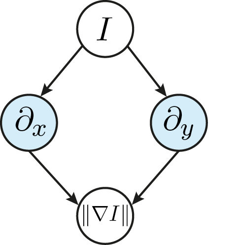
As you can see, the two filter responses can be calculated independently from each other. What is more: they both use the same image as input. We can exploit this fact and write a specialized kernel which calculates two filter responses at the same time.
float2 filter_sum_double_3x3(read_only image2d_t imgIn,
                             constant float* filterKernel1,
                             constant float* filterKernel2,
                             const int2 coordBase,
                             const int border)
{
    float2 sum = (float2)(0.0f, 0.0f);
    const int rows = get_image_height(imgIn);
    const int cols = get_image_width(imgIn);
    int2 coordCurrent;
    int2 coordBorder;
    float color;

    // Image patch is row-wise accessed
    // Filter kernel is centred in the middle
    #pragma unroll
    for (int y = -ROWS_HALF_3x3; y <= ROWS_HALF_3x3; ++y)       // Start at the top left corner of the filter
    {
        coordCurrent.y = coordBase.y + y;
        #pragma unroll
        for (int x = -COLS_HALF_3x3; x <= COLS_HALF_3x3; ++x)   // And end at the bottom right corner
        {
            coordCurrent.x = coordBase.x + x;
            coordBorder = borderCoordinate(coordCurrent, rows, cols, border);
            color = read_imagef(imgIn, sampler, coordBorder).x;

            const int idx = (y + ROWS_HALF_3x3) * COLS_3x3 + x + COLS_HALF_3x3;
            sum.x += color * filterKernel1[idx];
            sum.y += color * filterKernel2[idx];
        }
    }

    return sum;
}

kernel void filter_double_3x3(read_only image2d_t imgIn,
                              write_only image2d_t imgOut1,
                              write_only image2d_t imgOut2,
                              constant float* filterKernel1,
                              constant float* filterKernel2,
                              const int border)
{
    int2 coordBase = (int2)(get_global_id(0), get_global_id(1));

    float2 sum = filter_sum_double_3x3(imgIn, filterKernel1, filterKernel2, coordBase, border);

    write_imagef(imgOut1, coordBase, sum.x);
    write_imagef(imgOut2, coordBase, sum.y);
}
The filter_sum_double_3x3() function now takes two filter definitions as a parameter (lines 2–3) and returns both responses in a float2 variable which are saved in the two output images (lines 47–48). There is not more about it and it is not surprising that this test case outperforms the single approach. Of course, this works only with filters which do not need to be calculated sequentially.
Predefined
When we already know the precise filter definition like in \eqref{eq:FilterOptimization_ScharrFilter} we could use the information and write a kernel which is specialized for this filter. We don't have to pass the filter definition as an argument anymore and, more importantly, it is now possible to optimize based on the concrete filter values. In case of the Scharr filter, we can exploit the fact that we have three zero entries. There is no point in multiplying these entries with the image value or even loading the affected image pixels into the private memory of the work-item. An optimized kernel for \(\partial_x\) may look like
float filter_sum_single_Gx_3x3(read_only image2d_t imgIn,
                               const int2 coordBase,
                               const int border)
{
    float sum = 0.0f;
    const int rows = get_image_height(imgIn);
    const int cols = get_image_width(imgIn);
    int2 coordCurrent;
    int2 coordBorder;
    float color;

	coordCurrent.y = coordBase.y + -1;
	coordCurrent.x = coordBase.x + -1;
	coordBorder = borderCoordinate(coordCurrent, rows, cols, border);
	color = read_imagef(imgIn, sampler, coordBorder).x;
	sum += color * -3.0f;
	coordCurrent.x = coordBase.x + 1;
	coordBorder = borderCoordinate(coordCurrent, rows, cols, border);
	color = read_imagef(imgIn, sampler, coordBorder).x;
	sum += color * 3.0f;
	coordCurrent.y = coordBase.y;
	coordCurrent.x = coordBase.x + -1;
	coordBorder = borderCoordinate(coordCurrent, rows, cols, border);
	color = read_imagef(imgIn, sampler, coordBorder).x;
	sum += color * -10.0f;
	coordCurrent.x = coordBase.x + 1;
	coordBorder = borderCoordinate(coordCurrent, rows, cols, border);
	color = read_imagef(imgIn, sampler, coordBorder).x;
	sum += color * 10.0f;
	coordCurrent.y = coordBase.y + 1;
	coordCurrent.x = coordBase.x + -1;
	coordBorder = borderCoordinate(coordCurrent, rows, cols, border);
	color = read_imagef(imgIn, sampler, coordBorder).x;
	sum += color * -3.0f;
	coordCurrent.x = coordBase.x + 1;
	coordBorder = borderCoordinate(coordCurrent, rows, cols, border);
	color = read_imagef(imgIn, sampler, coordBorder).x;
	sum += color * 3.0f;

    return sum;
}
This is probably one of the most explicit forms possible. No for loops anymore, every operation is written down and the filter values are simple literals6. As you may have noticed, only six image values are loaded instead of nine as before. This limits memory transfer down to its minimum.
The benchmark results show that the approach performs very well and is relatively independent of the filter size. This is not surprising though since also larger Scharr filters have only six non-zero entries.
Selected combinations
Testing combinations of the approaches shown so far can easily turn into an endless story since so many combinations are possible. To keep things simple, I want to focus on three different questions:
- Does local memory also help to improve in the double approach? Would be weird if not.
- How does the double approach perform with predefined filters?
- Does local memory help with predefined filters?
As you can see, I already abandoned separate filters since their behaviour is just not appropriate for my application. The following chart contains a few more results to answer the questions.
As expected, the double approach does also benefit from local memory and works well with predefined filters. No surprises here. But note that local memory does not work well together with predefined filters, neither in the single nor in the double approach. Of course, since only six image values are loaded regardless of the filter size a huge difference is not to be expected. But it is interesting that the results with local memory are even worse (in both cases).
After all this testing, are there some general rules to infer? If you ask...
- Whenever possible, calculate the response of two filters at the same time using the double approach.
- If you know the exact filter definition in advance, write a specialized kernel just for that filter but test if using local memory speeds up your application.
- In all other common cases make sure to use local memory for filter sizes \(> 3 \times 3\).
- Don't forget that all results are highly application-, hardware- and software-specific. Take the time and test it on your own hardware and in your scenario.
List of attached files:
- FilterOptimization_LocalComparison.nb [PDF] (Mathematica notebook with the test data for the detailed local comparison between the two and one loop approach)
- FilterOptimization_SeparationExample.nb [PDF] (Mathematica notebook which contains the full separation example)
- FilterOptimization_BoxPlotPreparation.nb [PDF] (Mathematica notebook which calculates the statistical data for the box plot in the separation approach)